ChatGPT에 이은.. 쌓인 논문/공부 부채 상환하기 2편: Diffusion Models
본인의 전공 도메인이 Vision이 아닌 데다, 수식도 너무 많아 어떤 논문부터 공부해야 할지 고민하던 중, DDPM(Ho et al., 2020)부터 살펴보기로 결정!
완벽하게 수식을 이해하기보다 직관적으로 납득하는 방식으로 리뷰함
Diffusion Models
(DDPM 논문과 함께 위 블로그 포스팅을 참고.. OpenAI Researcher 분이 운영하시는 좋은 블로그)
)1.
Diffusion Model이란?
•
원본 이미지에 Gaussian Noise를 점진적으로 추가하여 Noisy한 이미지를 생성하고 (Forward Process),
•
생성한 Noisy한 이미지로부터 원본 이미지를 복원하는 방식(Reverse Process)으로 학습되는 생성 모델
•
(Gaussian 분포를 따르는 Latent를 샘플링하여 원본 이미지를 복원+Variational Lower Bound를 활용하는 VAE의 Multi-Step 버전으로 생각할 수 있지 않을까?)
2.
Forward Process,
•
Step에 걸쳐 원본 이미지 에 작은 양의 Gaussian Noise를 추가
•
추가하는 Noise의 양은 Variance 값인 에 의해 결정
•
Step 에서의 조건부 확률은 위와 같이 표현할 수 있는데,
•
다음과 같은 Gaussian Merge 과정을 통해 유도할 수 있음 (주목: Reverse Process 파트에서 다시 언급됨)
주목: Reverse Process 파트에서 다시 언급됨)3.
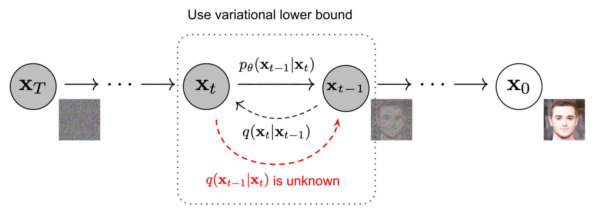
Reverse Process,
•
만약, 가 충분히 작다면 역시 Gaussian으로 생각할 수 있으며,
•
를 직접 도출하기는 쉽지 않으므로 Diffusion Model, 을 활용하여 근사값 를 도출함
•
VAE와 유사하게 의 Negative Log Likelihood에 Variational Lower Bound를 적용하면, 아래와 같이 풀이할 수 있고,
•
결국, Diffusion Model의 학습에서 Optimize하는 Loss는 다음과 같음
•
•
(Forward Process의 마지막 수식, 에 의하여)
•
다시 로 돌아와서, 결국 Diffusion Model의 학습 Objective는 각 Step, t별로 를 에 근사시키는 것으로 생각할 수 있음
DDPM: Denoising Diffusion Probabilistic Models

(참고할 만한 좋은 Codes)
•
DDPM은 의 를 학습되지 않는 상수로 설정
◦
실험적으로 가 일 때와 일 때, 비슷한 결과를 보인다고 함
•
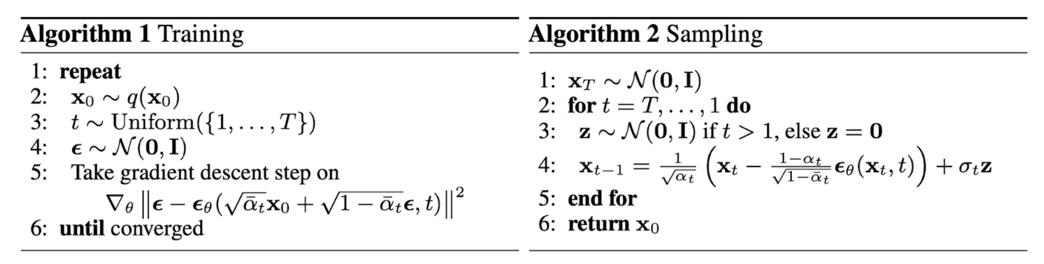
또한, 의 를 아래와 같이 Parameterization함
•
Parameterization 결과로 얻은 의 Weighting Term을 제거하여, 다음과 같은 최종 Training & Sampling 알고리즘을 제안